NeoSpace - Shaping the Next Era of Banking with AI

The Second Wave of Data-Driven DecisionsHitting the Wall: How Deep Learning Shatters the Limits of Classic Machine Learning

“We do not describe the world we see; we see the world we can describe.” R. D. Laing

The era of digital transformation brought an undeniable force that pushed companies to redesign their customers’ experience. As products and journeys moved to apps, web, and automated service channels, the business started producing a lot of event data: each client’s interaction with a company – opening the app, browsing a product, simulating a loan, making an investment, booking a flight, buying insurance, making a purchase, paying a bill, contacting support, or changing personal data – all started generating data entries in the company’s databases.

Naturally, seeing in that data crucial information to support predictions and inferences about the customers’ future behaviour, companies began to invest in scalable data infrastructure and ingestion pipelines, consolidating data into data lakes in order to create a reliable foundation where data from several systems could be stored, standardized, and made usable. The major lines of research in Machine Learning, however, used to see raw data as being too noisy and too granular to drive decisions directly. Moreover, there was a general lack of computational power to process streams of events into prediction engines. So, data scientists and engineers began transforming those raw events into “features”, which were to be seen as compact, more “decision-ready” signals that summarize customer behaviour.

Instead of the raw data, businesses started relying on data aggregations like averages, standard deviations, maxima, minima, data frequency and recency. In this way, feature stores became ubiquitous, constituting the operational layer organizing those data aggregations so they could be reused consistently across teams and models, keeping them up to date at the right frequency, and guaranteeing that they were applied in production in the same way they were defined and applied during training.

Not rarely, organizations would build an entire ecosystem of specialized models – sometimes, even hundreds of them – tailored to specific products, channels, objectives, and segments. The orchestration of such ecosystems began to rely on parameterization rules which became the decision layers that turned predictions into concrete actions by combining the Machine Learning outputs with business rules, policy constraints, budget and exposure limits. A “industrial” pipeline was born: events became features, features were fed into models, models outputs met business rules to become offers and, finally, more recently, AI agents based on large language models combined with companies apps or general communication apps became the final layer through which the offers finally reach the client.

However, this reliance on human-engineered features, while providing interpretability and alignment with established business logic, inherently restricts the model's exploratory potential. Because these features are designed based on prior business knowledge, they effectively act as a filter that reinforces existing operational paradigms, often shielding the model from identifying novel, non-obvious causal drivers. This 'knowledge-imprinting' can create a bias toward confirming what is already known, potentially overlooking complex sets of weak causal signals that, if analyzed holistically without the constraint of manual feature engineering, could coalesce into actionable, high-value insights previously hidden within the data noise.

This landscape of data-driven decision making still constitutes the present state of most companies. It requires huge investments and constant specialized effort in defining rules. Even so, this pipeline is very slow to react to structural market changes, is much less hyperpersonalized than it would seem to be at a first glance, and is far from being as accurate as the information embedded in the original, raw event data, would allow it to be.

What we have described so far is, essentially, the classic Machine Learning paradigm operating at industrial scale: raw events are transformed into aggregated features, features are organized in features stores, models consume those features, and decision layers orchestrate outputs through rules and constraints. Modern Deep Learning, however, changes the default approach by making the raw event stream – not its aggregations – the central asset. When models can learn directly from transactional histories, behavioural sequences, and unaggregated interactions (including text), they tend to react faster to structural market shifts, enable truly real-time predictions, and achieve better predictive performance.

Let the data speak

“The description is not the described.”

– Jiddu Krishnamurti

One of the major perspective shifts from classic Machine Learning to modern Deep Learning concerns how much do we really need to “teach” the model or, more specifically, how much models benefit from our field knowledge of a given field versus learning it for itself.

A groundbreaking example comes from DeepMind’s AlphaZero. Before AlphaZero, top-performing chess engines looked a lot like the “industrial” pipeline we described: you first handcrafted representations of what mattered (material balance, pawn structure, king safety, mobility, and many other heuristics), then used search procedures (alpha-beta pruning, extensive lookahead) guided by those signals. Even with superhuman brute-force capacity, the engine was still navigating the game through a human-designed description of what “good chess” looks like.

AlphaZero was a counterpoint. It was built on a deceptively simple premise: don’t tell the model what a “good position” is. Don’t hardcode centuries of chess understanding. Don’t build a feature catalogue of “what matters”. Give the system only the rules of the game, the objective (win and what win means), and the ability to generate experience by playing against itself. What happened is that AlphaZero learned two things at once:

A rich representation of the state (what aspects of the board position are important, and how they combine), and
A decision policy (which moves to consider and prioritize), guided by feedback from outcomes.

In other words, it learned how to describe the world in a way that makes winning possible – rather than inheriting a human description.

AlphaZero convincingly defeated Stockfish (at the time the most advanced chess-playing system) in a 100–game match scoring 28 wins, 72 draws, and 0 losses. Since then, Stockfish evolved by incorporating components (e.g., NNUE) to reduce search complexity by learning meaningful representations.

The same shift applies beyond board games. A classic credit scoring model, for example, would be trained on several data aggregations like averages, standard deviations, maxima/minima, counts, frequency/recency, rolling windows, handpicked ratios, and so on. But it is the data that gave rise to those aggregations what a deep model would most benefit from. Instead of being restricted to the statistics we chose, the model can search for richer structure in sequences and interactions: not just how often something happened, but in which order, under which context, how patterns evolve, and which combinations matter – including combinations no one would ever think to hand-engineer.

There are several ways in which aggregation can hurt learning: 1 Curiously enough, human chess playing is not actually based on huge lookahead capacities; obviously, some lookahead ability is involved, but elite chess players are not brute-force calculators so much as fast recognizers. World champion Vladimir Kramnik says that, beyond “textbook” play, at grandmaster level, “sometimes you do not have to think that much” – the move can arrive almost automatically. Classic cognitive research matches this testimony: de Groot’s protocol studies found no big differences in depth-of-search statistics, and Chase & Simon summarize that masters often consider “about the same number of possibilities – perhaps, even fewer” than weaker players, but are dramatically better at generating the right candidate moves to analyse. However, being unable to directly teach those board-level internal representations (the tacit motifs and positional impressions that masters acquire over years), we have to approximate them. And this leads to handcrafted evaluation functions, like material weights, king safety terms, pawn-structure penalties, mobility bonuses, and countless other human-designed heuristics. So, classic engines try to compensate for representational limitations with brute computation.

Information loss (irreversibility). In general, it is impossible to recover the original data from its aggregations.
Inexpressiveness for certain modalities. Some inputs are inherently hard to aggregate meaningfully, like raw text. Yet, these can be decisive for a task (think of the role of a client’s WhatsApp interaction with a company in predicting the client’s propensity to buy a certain product).
Underrepresentation of sparsity. When data is aggregated over time or events, sparse data (such as, in the above example of a credit scoring model, the events of a client with few transactions) tends to be “washed out” of the dataset, leading to very poor performance of the model in those cases.
Injected bias. More subtle is the fact that, by choosing how data is aggregated, we are imposing to the model a bias, that is, a certain view of the world that reflects what is generally called “field knowledge”. While this may seem a good thing, it might block exactly what we want from a predictive model: a genuinely new way to look at the data.
Cost and maintenance of feature stores. Building and maintaining a feature store is expensive and specialized work, requiring a team that understands both the modeling techniques as well as the relevant knowledge domain. This is especially true when a new data source is to be introduced, since it needs to be deeply evaluated and studied before meaningful new aggregations are added to the store.
Domain specificities. Aggregation choices and strategies that work for a certain domain do not work for other ones (for instance, aggregation windows typical for a credit scoring model will, in general, not perform well for a CTR model).
Structural changes of the market. It is not uncommon for data aggregations to work well during a certain period of time but to become not as effective (or even totally ineffective) in other periods of time due to relevant novelties that may cause a structural change in a prediction’s task.
Temporal and Structural Rigidity. Traditional aggregation relies on fixed temporal windows (e.g., 30-day moving averages), which implicitly assume a static relationship between the feature and the target. This creates a "brittle" model that struggles to adapt to rapid changes in consumer behavior or market shifts. When the underlying market dynamics change, these hard-coded aggregations often fail, as they lack the flexibility to redefine their own predictive scope in real-time.
Loss of Behavioral Volatility (The "Mean Tyranny"). Aggregation methods like averages or medians inherently smooth out the data, prioritizing stability over precision. In many domains — such as fraud detection or credit scoring — the most predictive signal is not the "typical" behavior, but rather the sudden, sharp deviation or the isolated "spike" in activity. By condensing these events into statistical summaries, we effectively "wash out" the very behavioral signatures that signal an impending change in risk or propensity, rendering the model insensitive to critical, high-impact anomalies.
Knowledge-Imprinting and Causal Blindness. By forcing data into predefined feature categories, we essentially constrain the model to "confirm" existing business hypotheses rather than allowing it to discover ground-truth patterns. This "knowledge-imprinting" acts as a filter that reinforces established operational paradigms, shielding the model from identifying novel, non-obvious causal drivers. Consequently, we may overlook complex sets of weak, fragmented causal signals that, if analyzed holistically without the constraint of manual feature engineering, could coalesce into new, high-value insights.

2 Click-Through Rate models, designed to predict the likelihood of a user clicking on a given link.Interesting illustrations of this last point are the introduction, in Brazil, of Pix transactions (instant interbank transactions that have become the dominant payment method, capturing approximately 50% of all transactions and facilitating a total volume of nearly $7 trillion throughout 2025 , and the recent and sharp rise of online betting apps. Such novelties completely reshaped the landscape of credit default prediction in the country.

An adequately designed and trained deep model should completely remove those kinds of worries. Structural changes in the prediction problem are to be naturally incorporated and dealt with, because shifting structural behavior is captured in real time through the raw data itself. The absence of aggregation periods leads to real time predictions (a single credit card transaction may instantly trigger a reevaluation of its available credit limit, for example).

So far, we have been looking only at the model inputs, but a similar perspective change also applies to the outputs. Indeed, in the classic paradigm, we are actually using proxies twice: once when features are taken in place of raw data; and twice when customer-level decisions are collapsed into proxy scores that require a separate rules layer to become an action. In other words, not only the model should learn directly from the raw event stream, but it should also output structured, customer-specific decisions.

Let the model act

“Well done is better than well said.”

– Benjamin Franklin

If we are to let data speak, we also have to let the model answer in the language of action. In the classic setup, the model’s output is still an abstraction: scores that must be interpreted, translated into thresholds, policy tables, and manual rules. But that translation layer is actually a second model that is being fed aggregated data, because the scores are nothing but a very compressed and simplified version of the model’s rich representations that were learned from the raw event stream. So, beyond the scores, we must let the model translate those representations into hyper-personalized actions.

In a modern credit architecture, the model should no longer answer a narrow predictive question such as “What is this customer’s probability of default over the next 12 months?” and then rely on downstream rules, policy tables, and manual parameterization to convert that estimate into action. Instead, the system should directly solve a constrained decision problem and produce an action object: a structured, auditable output that specifies what should be done for this specific customer, given the institution’s economic objectives, capital constraints, and regulatory boundaries.

In this setting, the model is not merely predicting risk; it is optimizing a customer-level decision under explicit objectives — for example, maximizing expected risk-adjusted return or MFL minus cost of capital — subject to portfolio, regulatory, and fairness constraints.

Concretely, rather than a single credit score, the system would output:

A recommended credit line (or line adjustment), accompanied by uncertainty estimates and capital consumption implications.
Pricing terms selected to optimize expected margin net of risk and funding costs, consistent with the institution’s risk appetite and customer lifetime value considerations.
Product and channel selection: whether the next best action is a limit increase, balance transfer, secured product migration, restructuring proposal, or no offer at all — and whether it should be delivered digitally, through push notification, email, or via a human agent.
Timing and pacing: when to trigger the intervention, taking into account behavioral signals (e.g., post-salary inflow, transaction patterns, service interactions) and dynamic portfolio conditions.
Guardrail-aware constraints: outputs that already respect exposure limits, concentration thresholds, regulatory requirements, fairness metrics, stress-scenario capital limits, and commercial budget caps.

Crucially, this action object should not be static. It must be embedded in a continuous learning loop, where realized outcomes — acceptance, repayment behavior, attrition, and profitability — feed back into the policy engine. The system must distinguish between natural customer behavior and behavior induced by intervention, incorporating causal or uplift mechanisms to ensure that recommended actions generate incremental value rather than merely predict it.

Under this paradigm, credit modeling evolves from score estimation to policy optimization. The output is no longer a number that requires translation into action; it is a decision framework that integrates risk, return, customer experience, and portfolio coherence into a single, executable object.

In other words, the model’s output is closer to a hyper-personalized credit policy than to a score. For one customer, the best decision might be “reduce exposure but improve retention”: propose a lower limit increase (or none), offer a restructuring plan, and choose empathetic messaging to protect NPS. For another, it might be “increase exposure aggressively”: a higher limit with a lower rate, because the model sees high stability, strong3 Net Promoter Score, a customer loyalty score which is a key indicator for customer satisfaction and brand advocacy.Cashflow patterns, and strong long-term value. The point is that these are not “segments”, but individual policies generated from the customer’s trajectory.

If the system is trained only to predict default, it may optimize for avoiding loss, but often at the cost of declining profitable customers and/or harming experience. But if the objective is defined at the right level, say, “maximize expected lifetime contribution” (revenue minus loss and cost) while maintaining NPS and long-term retention, the model can learn decisions that trade off risk, margin, and relationship quality directly. The score may be seen as an internal latent signal, but it is not the product. The product is the action: the right limit, terms, offer, timing, and message for this customer, under explicit governance constraints.

A model with such capabilities can be seen as the foundational AI brain of the modern enterprise. We call it a Large Data Model.

Large Data Model – LDMA Foundational AI Brain

“It is the pattern [...] which is the touchstone of our personal identity. [...] We are but whirlpoolsin a river of ever-flowing water.We are not stuff that abides, but patterns that perpetuate themselves. A pattern is a message,and may be transmitted as a message.”

– Norbert Wiener

A Large Data Model (LDM) is a transformer-based deep architecture pre-trained from scratch on the raw operational data of a business system. Here, “business system” is used in a broad sense: it may refer to a bank, hospital, telecom operator, insurance company, law firm, energy company, sports organization, university, or any ecosystem of interacting entities whose activities generate structured event data.Unlike traditional machine learning models trained on curated feature tables, an LDM is trained directly on systems-of-record and interaction logs: customer profile updates, purchases, transactions, digital sessions, claims, tickets, CRM interactions, operational events, and other state transitions. The model ingests these heterogeneous, time-ordered signals and learns the joint dynamics of customers, products, operations, and organizational decisions. In practice, pretraining is typically self-supervised, enabling the model to learn a compressed representation of the evolving enterprise state without requiring task-specific labels.

An LDM is not a language model. Its purpose is neither text generation nor human communication. Rather, it is a foundation model for the enterprise itself. Through large-scale pretraining on raw business data, it acquires a generalized representation of how the company and its ecosystem behave over time. After post-training or task-specific adaptation, this representation can be leveraged to power predictions and decision-support tasks such as risk assessment, demand forecasting, churn prediction, pricing, fraud detection, capital allocation, and next-best-action policies.

In this sense, an LDM serves as the company’s foundational intelligence layer: a unified model of its operational memory and behavioral dynamics.

Operational impact

With all our clients so far, the Large Data Model paradigm consistently demonstrates substantial performance improvements over traditional machine learning approaches built on manually engineered features. In more than 12 predictive and decision-support tasks across large-scale enterprise datasets — particularly in data-intensive sectors such as financial services — models trained directly on raw event streams achieved performance gains typically ranging between 15% and 60% relative improvement compared to conventional tree-based machine learning pipelines or narrowly fine-tuned task-specific models.

These improvements appear consistently across tasks that involve complex behavioral dynamics, where long-range temporal dependencies, sparse signals, and heterogeneous data modalities play a decisive role. Early experiments conducted in other domains with similarly rich operational data show promising results that follow similar patterns.Importantly, these gains are not limited to predictive accuracy alone. Because LDMs learn unified representations of operational behavior, they often reduce the need for maintaining large ecosystems of specialized models and handcrafted features. This leads not only to stronger predictive signals but also to a simpler and more adaptable modeling infrastructure, particularly in environments where customer behavior, market conditions, or product dynamics evolve rapidly.

Pre-train: building understanding and perception

During the pre-train phase of the LDM the model learns deep interconnections between the company’s data. These interconnections are expected to be quite intricate and the mathematics behind them show that, indeed, they usually have “high order”, are quite “implicit”, or depend on complex geometric transformations to be exposed (see Section “Local Fusion Layers”). It is also important to note that, before pre-train, the model’s weights are random, that is, there is no prior training of the model on generic tabular data and the only data the model ever sees is the company’s data.

In order to have a better grasp of the pre-training, let us deal with a concrete example. Our “company” will be a fictional tier-1 Telecom whose core databases include, among others, data about network sessions and performance, call detail records (CDRs), radio measurements and cell-level KPIs, device and SIM inventory, plan activations and changes, billing and invoice events, payment and delinquency events, customer care interactions (IVR, chat, tickets, complaints), field technician visits, roaming events, marketing touches, and churn/reactivation history. So, given a customer (or household / account) and a certain time range, the model would see a sequence of events like the one below (for illustration purposes, the dataset entries are shown in a simplified form):

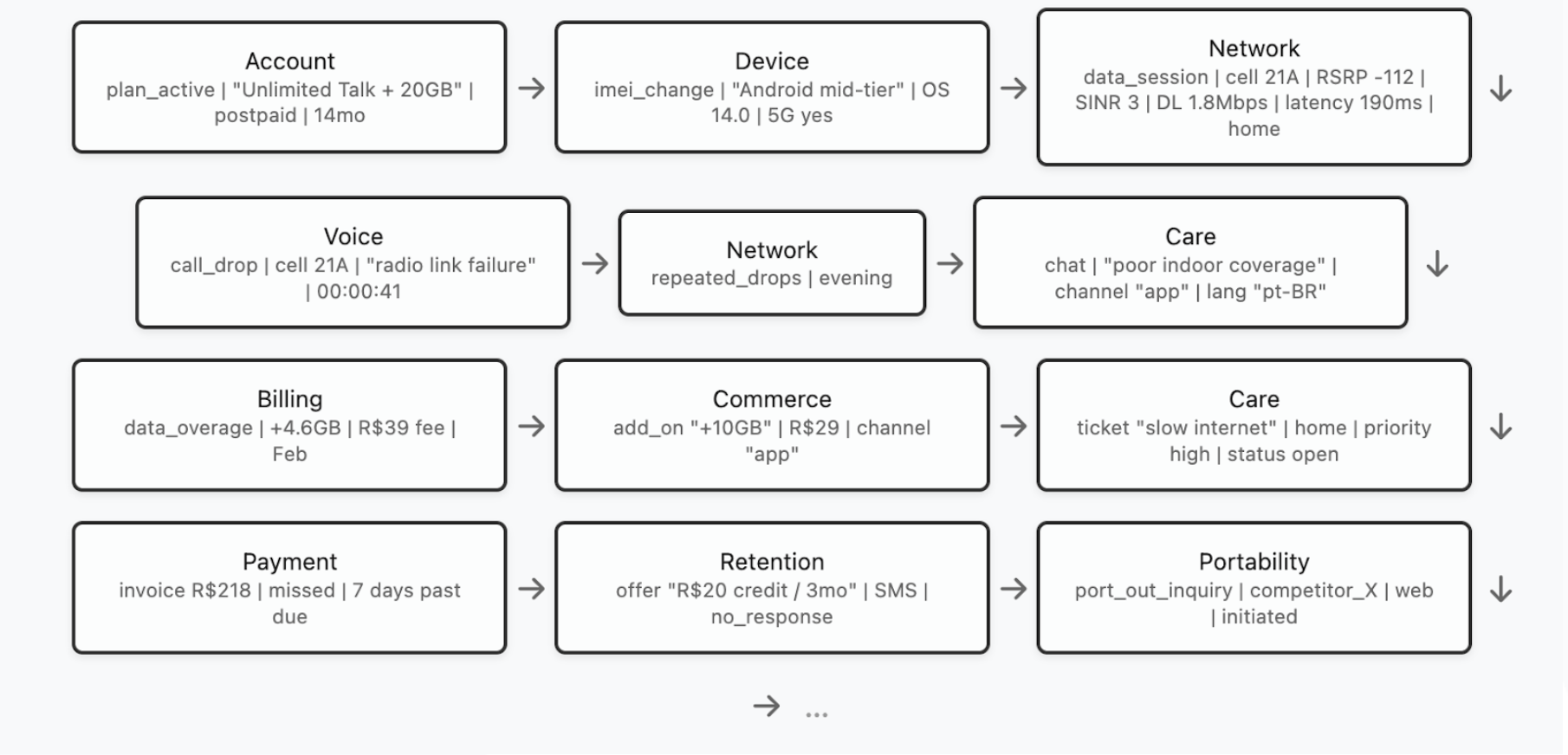
Now, the model must be trained to understand each customer’s story so that, later, we can teach it how to intervene in them. Pre-training is a self-supervised phase, which means that no human labels are required. Instead, the goal of the model is to learn to predict future events from past ones. More precisely, by feeding the LDM the events that happened at times , we expect the LDM to be able to predict at least the customer’s next event (ideally, the LDM should be trained to predict a few next events of the customer). So, if the model sees the above trajectory

[...] → high latency → voice call drop → repeated network drops → ?

it is supposed to predict which event is likely the next one: a support call? A plan downgrade? A port-out request? A device swap? It must also predict every specific aspect of the next event. So, in this example, the model should predict that the next event is more likely to be a “chat” complaint of “poor indoor coverage”, through the “app” channel, in the “pt-BR” language. This forces the model to understand, among many other things, service quality degradation patterns, customer behaviour under friction, and the interplay between network experience and commercial outcomes.

Besides the next event(s) prediction, there are other objectives that help the model to create expressive representations of the datasets. With masked event modeling, for example, the model is supposed to predict a missing part of an event. For instance, asking the model to infer the missing throughput value in the event

it must learn to understand radio conditions, congestion patterns, device capability constraints, location/time effects, and typical ranges for similar customers and cells.

After seeing millions of customers' journeys, the model will encounter rare incidents, edge cases, roaming quirks, device firmware regressions, seasonal congestion, protocol changes across years, market campaigns, staff practice differences… it learns patterns no single analyst could observe in a lifetime. Even more, it is able to find interconnections between such patterns that are way beyond human capability. Perception emerges as the model understands usage archetypes, long-term customer behaviour patterns, unusual trajectory deviations, which network signatures cluster together, how service quality evolves by geography and time, how interventions change trajectories, what patterns precede churn, delinquency, or repeated complaints, etc. The model has now profoundly learned the structure of customer experience and service delivery inside that telco.

Differently from pre-training, the post-training phase of an LDM requires creating targets that are particularly suited to the task that we expect the model to perform. We divide post-training into two categories: the Predictive Post-Training and the Prescriptive Post-Training.

Predictive Post-train: building forecasting power

Predictive post-training turns pretrained representations into measures: scores, rankings, embeddings, forecasts, segments, financial results and other non-executing outputs. By design, a predictive post-trained LDM does not decide what to do — it summarizes and anticipates what is likely to happen, and therefore still requires an external policy layer (thresholds, capacity rules, eligibility tables) to convert predictions into actions.

Operationally, predictive post-training requires labeling the event stream. For each entity (customer / account / household) and timestamp t, we create targets defined over a look-ahead window [t, t + Δ]. Examples in a Telecom setting include:

churn/port-out within 30/60/90 days,
delinquency in the next billing cycle,
repeat care contact within 7 days,
complaint escalation within 14 days,
persistent QoE degradation over the next week.

Each target is built by scanning the raw logs forward from t and marking whether the event(s) of interest occur in the chosen horizon. The model is then trained to map the historical trajectory up to t into these labels (often many at once in a multi-target setup). Because this phase builds on strong pretrained representations, a single post-training pass can cover multiple horizons and outcomes without requiring a dedicated model per objective.

Prescriptive Post-train: building judgement

Prescriptive post-training goes one step further: instead of producing measurements that a separate policy layer must translate into decisions, the model is trained to output the decision itself (as described in “Let the model act”). It "absorbs" the policy layer into the model by directly optimizing the organization’s final objective (profit, retention, NPS, cost-to-serve) under explicit constraints.

Enabling this kind of training requires a different kind of supervision. Rather than labels like “churn in 60 days”, we build training examples of the form:

Context: the customer trajectory up to time tAction: what the company did at t (say, offer / terms / channel / timing / message / “nothing”)Outcome: what happened after that action over a horizon [t, t + Δ] (margin, loss, churn avoided, complaints, NPS proxies, etc.)

From these outcomes we define a reward/utility that matches the business objective (for example, expected contribution = revenue − loss − service cost, with penalties for policy violations and experience harm). The model is then trained to produce actions that maximize this utility subject to guardrails (budget, exposure, eligibility, regulatory constraints). In practice, this can be implemented as offline policy learning: learning from logged decisions and their downstream outcomes, with techniques that correct for the fact that historical actions were chosen by an existing policy (so the model doesn’t merely imitate yesterday’s rules).So, while predictive post-training learns to forecast the future, prescriptive post-training learns the policy that acts on the future. The external policy layer is no longer a separate system, but a learned component of the model.

Architecture and Data Interface

An LDM is designed to transform heterogeneous enterprise records – transactions, interactions, operational logs, and text – into unified latent states that support prediction and decisioning. The central modeling object is an event stream: for each entity (that is, customer, account, household, device), we observe a time-ordered sequence of events generated by multiple source systems.

Throughout this section, we assume the data can be represented (or converted) into an event-based format. Concretely, each event contains: (i) one or more entity identifiers (the join keys that define “who” the event belongs to), (ii) an event time (the ordering key that defines “when” it happened), and (iii) a set of typed fields (numeric, categorical, timestamps, free text, and even images or other modalities). Non-event datasets (e.g., slowly changing dimensions or snapshots) can be incorporated by projecting them into event updates or by attaching them as contextual side information.

At a high level, the architecture has five functional blocks:

Field encoders that map each raw field into vectors in representation spaces;
Local fusion layers that model interactions among fields within the same event;
Temporal backbone that models long-range dependencies across the event sequence;
Spatial backbone that captures dependencies across entities (e.g., households, merchants, devices, cells);
Latent-state processor that converts the resulting entity state into task outputs (scores, forecasts, or structured action objects), while enforcing governance constraints through training objectives and/or constrained decoding.

Embedding Layers

Embedding data is the process of taking data in its original type (say, a float, an integer, or a string) and representing it geometrically as a point in a Riemannian manifold. This Riemannian structure will later play a role in the model’s training, where geometric structures like angles, distances, geodesics, etc, can be explored in order to minimize the training objective function. Typically, the Riemannian manifold is taken as an n-dimensional Euclidean vector space with an arbitrarily chosen orthonormal basis; for simplicity, in what follows, we will stick to that case. So, roughly speaking, we can think of embedding data as the process that turns each data field in a client’s event into a vector that represents this data field.

If we leave aside the problem of choosing a meaningful geometry, embedding low/medium categorical features is very simple: one just has to associate to each category a randomly initialized vector. During training, the model must determine — or learn — each of those values in such a way that the role of the corresponding category in the task(s) performed by the model can be meaningfully expressed by its representation. This is typically called “learned embedding tables”.

Embedding free text is perhaps one the most well-explored types of embedding, due to the success of Large Language Models. The standard way to embed text is first to create a tokenizer (that is, an algorithm that converts pieces of text into integers, in such a way that text becomes a list of integers in a deterministic way) and then to associate a vector (with randomly chosen values in the beginning of training) to each such integer. In an LLM, this list of vectors passes through a Transformers architecture4 Although, depending on data structure, it is more adequate to use a product of negative curvature spaces (like hyperbolic space), positive curvature spaces (like projective spaces), and Lorentzian spaces (like de Sitter and anti de Sitter spaces).

Where a next token prediction will be used to train the model. In an LDM, we want to turn a given textual entry into a single vector that represents the entire text. That can be achieved by using a Transformers-like model as well, but with some pooling technique at the end: we may, for instance, take the mean of all predicted next tokens or, instead, take the last predicted token.

Embedding continuous scalar values remains substantially more challenging than token embedding and is still comparatively underexplored. In enterprise data, however, scalar quantities are not peripheral — they define the system’s state: balances, exposures, prices, limits, volumes, probabilities, latencies. A model that fails to represent numerical structure faithfully cannot build a coherent representation of the system’s dynamics.

Large Language Models illustrate this limitation clearly. Because they operate over discretized tokens and are not explicitly trained for algorithmic consistency, they often struggle with exact arithmetic, scale extrapolation, and magnitude sensitivity. Their embeddings do not enforce numerical invariants such as ordering preservation, monotonicity, or stability under affine transformations. In language modeling this may be tolerable; in enterprise modeling it is not.

A robust numeric encoding must therefore expose the intrinsic structure of continuous variables — sign, ordering, relative distance, and basic algebraic relations — while still allowing the model to capture dataset-specific regularities such as heavy-tailed distributions, characteristic scales, regime shifts, seasonality, and multi-frequency periodic components. In our experiments, a hybrid encoding that combines value-domain representations with spectral (Fourier-feature) embeddings performs consistently well, providing sensitivity to absolute magnitude while preserving resolution across multiple temporal and frequency scales. The same principle extends naturally to timestamp features, where periodic and hierarchical temporal structure must be made explicit.

In LDMs, numerical representation is not an auxiliary design choice; it is a structural requirement for modeling enterprise state transitions.

Local fusion layers

“— It is about how entities manifest themselves to one another. It is about relations.”

— Carlo Rovelli

Up to this point, we have treated an event as a collection of independent fields. But a real enterprise record only becomes meaningful through within-event interactions: numbers condition how we interpret text; categorical context changes what a metric “means”; timestamps define which regimes are comparable; operational metadata alters the semantics of an observation.

Formally, consider an event Et for an entity at time t, with numeric fields {ni}, categorical fields {cj} timestamps {tk}, and unstructured fields {sl} (text, images, etc.). After the embedding layer, we obtain a set of embedded vectors {Ni}, {Cj}, {Tk}, {Sl}.

A local fusion layer maps this heterogeneous set into a single event representation {Zt} — which we will call the entity's token at time t — that captures how the fields jointly define the event’s state. This is the first place where the model can express statements like: “this throughput value is alarming given this device capability, this cell congestion, and this location context” — not as a rule, but as a learned interaction.

A concrete example makes the need obvious. Suppose an event is a radiology exam record: the patient’s complaint and clinical history (text), scan protocol (categorical + numeric), contrast usage (categorical), image slices (vision modality), and the radiologist report (text). Interpreting the images without conditioning on protocol and context is fundamentally ill-posed: the same pixel pattern can mean different things depending on acquisition settings and clinical priors. The fusion layer is where the model learns these conditional dependencies, aligning modalities into a coherent event-level meaning.

In domains like CTR modeling (and more generally high-dimensional tabular decisioning), it is common to describe interaction modeling as either explicit or implicit. Explicit interaction layers (e.g., cross layers/ polynomial feature crosses) deliberately construct (usually, low to mid order) combinations of fields. They are strong baselines because they efficiently capture “if A and B then …” patterns and often improve sample efficiency on sparse tabular data.

While explicit crosses are effective, they hide an important limitation: they typically assume that multiplying coordinates in an arbitrary basis is a faithful notion of “interaction.” But embeddings are not raw measurements; they live in representation spaces whose geometry is learned and whose coordinates are not semantically privileged. Two consequences follow:

Basis sensitivity. A polynomial cross is not invariant to reparameterizations of the embedding space. The same semantic configuration can look different under an equivalent rotation/scaling of coordinates, yet the cross layer will respond differently.
Modality mismatch. Event fields come from fundamentally different encoders (numeric, categorical, text, image). Naively combining them through coordinate-wise algebra can overweight whichever encoder produces higher-variance activations, unless the fusion mechanism learns a metric-aware alignment.

For this reason, a robust local fusion block should be understood as learning a geometry for interaction, not merely stacking algebraic feature products. In our setup, quaternionic and gyrovector spaces are used so that the fusion operator treats representations as living in a latent space where meaningful combination corresponds to “structured reorientation”: signals are transformed in a way that separates “how strong” a component is from “in which direction” it points. In this way, interactions emerge as learned rotations (isometries) and controlled rescalings that align compatible factors and decorrelate conflicting ones.

Intuitively, instead of asking the model to discover structure through coordinate-wise multiplications in an arbitrary basis, we let it learn how event information should be rigidly moved through representation space, so that relative angles, phase-like relationships, and norm-preserving mixing become the primitives of fusion before projecting back into the model’s working dimension. This makes the interaction mechanism far less dependent on the accidental choice of coordinates and more faithful to the idea that what matters in fusion is alignment, orientation, and invariant structure: a learned geometry for interaction.

Backbones

The temporal backbone is the component that turns a time-ordered stream of fused events into a contextualized trajectory and a current latent state for each entity. Its job is not merely to “remember” what happened, but to learn how past interactions condition the meaning of the present.

The temporal backbone consumes a sequence of event tokens {Z1, Z2, …, Zn}, where each token already represents an event with its intra-event interactions resolved (via the fusion layers). It outputs a current state vector that represents everything the model “knows” about the entity at time t. This representation must support prediction under causality: at time t, the latent state should depend only on events that happened at times.

Many enterprise dynamics are not purely temporal: they are also relational. Customers share households, devices, merchants, employers, location, etc. The spatial backbone captures this structure by modeling how an entity’s trajectory is shaped by its neighborhood in a broader system.

Although it is tempting to define a neighborhood purely topologically, by handcrafting rules for which entities are “related” (same segment, same region, similar profile), this quickly reintroduces the very bias we are trying to avoid: we hard-code what similarity should mean. A more robust approach is to treat neighborhood selection as a learned geometric problem. Each entity’s state at time t lives in the model’s latent space; proximity in that space defines a notion of “peer context” that can change over time as behavior changes. In practice, the spatial backbone operates as a bounded retrieval-and-attend mechanism: given the current state, it retrieves a small set of nearby states and cross-attends to them to produce a context-enriched state. This makes “who influences whom” an emergent property of training rather than an external design decision, while still allowing operational constraints such as time consistency and compute budgets to be enforced. The output is a single, fused latent state that carries both personal history (temporal backbone) and system position (spatial backbone), and that state becomes the interface through which the model produces forecasts or decisions downstream.

In a nutshell, the temporal backbone learns what happened and what it means now; the spatial backbone learns who is relevant right now. Both are learned, not prescribed.

Latent Space Processor

The latent-state processor is the “readout and control” stage: it takes the latent state produced by the backbones and converts it into operational outputs which are either measurements (predictions) or structured actions (interventions). This is where the architecture becomes business-facing: the processor defines what the model can say and, crucially, how directly it can act.

At time t, the processor receives the current entity’s state and, optionally, a set of relational context from the spatial backbone. It may also receive objective context (campaign goals, product constraints, budget caps, regulatory regime) so outputs are conditioned on the operating mode rather than hard-coded.

For predictive post-training, the processor maps latent state into outputs such as probabilities/risks over multiple horizons, forecasts (counts, amounts, usage), rankings (next best product, likely complaint topic), embeddings for retrieval/segmentation A key property of a good processor is multi-task consistency: a single latent state should support many outputs without requiring a separate model per objective. This is usually implemented as a shared trunk (the backbones) with multiple lightweight task heads (classification/regression/ranking heads) that can be extended as new targets are added.

For prescriptive use, the processor produces an action object rather than scalar scores. The object is structured (typed fields, discrete choices, numeric parameters) and designed to be directly consumable by downstream systems, even a Large Language Model (LLM). Outputs should optimize the organization’s utility (margin, retention, cost-to-serve, experience) rather than a proxy like default probability alone. Moreover, the processor should enforce guardrails at generation time. Practically, this can be done by constrained decoding (only valid actions can be produced), by penalty terms in training, and by a feasibility module that projects suggested actions onto the allowed policy set.

Orchestrating Decisions with LLM Interfaces

While an LDM produces structured decisions, these decisions must still be communicated and executed through the interfaces by which companies interact with their clients. In practice, this interface layer is increasingly mediated by Large Language Models (LLMs). In this architecture, the LDM acts as the system’s decision engine, generating structured action objects that encode what should be done for a specific customer under the organization’s economic objectives and policy constraints. The LLM, in turn, acts as the interaction layer that translates those decisions into contextualized communication and orchestrates their delivery through customer-facing channels such as apps, messaging platforms, call center tools, or digital agents.

In this division of roles, the LDM is responsible for reasoning over the company’s operational state and producing the optimal intervention, while the LLM functions as the vehicle that operationalizes the action. The LLM interprets the structured action object , including recommended products, pricing, timing, and messaging constraints, and generates the appropriate human-readable communication or workflow execution. Because the decision itself originates from the LDM, the LLM does not determine what action should be taken; it simply ensures that the decision reaches the client in a coherent, personalized, and channel-appropriate form. This separation preserves governance and auditability while enabling the flexibility of conversational interfaces.

In practice, this architecture resembles the separation between a control system and a communication layer: the LDM governs the policy of action, while the LLM governs how that policy is expressed and delivered. The result is a unified system in which predictive intelligence, decision optimization, and customer interaction operate as coordinated layers rather than independent subsystems.

NeoLDM's

Transformer Model

Documentation

Careers

NeoNews